
An Approach to Explaining Confidence Intervals When Estimating Average Values

Five fixed-radius circular plots in the same stand, arranged in three spatial layouts, are likely to have different average estimated values.
During natural resource inventories, we often estimate average values such as average basal area per acre, average volume per acre, or average tons per acre. An estimate of the average value provides valuable information, but we also want to have some idea of the uncertainty associated with that estimate. How much “confidence” can we place in the estimate? If you have little confidence in your estimate, are you willing to use $300,000 of your own money to buy a tract of timber? What would make you feel comfortable enough to justify the expenditure of $300,000? We want to measure enough of the population so that we can make an informed decision based on sample data for the problem we are trying to solve. We don’t want to measure more of the population than is needed. If we do measure more than is needed, we will have wasted resources and time. Of course, the amount of the population deemed enough to make an informed decision will likely vary among foresters; some will feel more comfortable than others with a smaller sample of the population.
A stand is a collection of trees managed together as a unit. We hardly ever measure an entire population—every tree in the stand—in a loblolly pine plantation, bottomland hardwood forest, or mixed pine-hardwood forest. We often measure a reduced portion of all trees in the stand; stated differently, we conduct a sample of a stand. Due to time, logistics, and costs, we can’t measure every tree. Therefore, we have uncertainty associated with our estimate of the true average tons per acre because we only have partial knowledge about our stand.
Inventories often are conducted using fixed-radius plots or point sampling (variable-radius plot sampling). Average values per acre are simply the average of all the plot or point estimates. For a particular sample size and protocol, there are many different ways in which plots/points of that “cruise” could be established spatially. Each different spatial layout of the plots will likely produce a different estimate of the true average tons per acre. This is sampling error, or variability, in our average estimates because we are measuring only a portion of the trees in our stand, leading to uncertainty about our individual average estimate obtained during an actual operational inventory. In other words, we are making direct measurements (the sample) on only a reduced portion of the population.
How many different ways can five fixed-radius circular plots be established without overlap in the stand pictured above? There are probably more than 100,000 ways. For all of the potential spatial layouts, the average value of the five plots would produce a valid estimate of, say, the true average basal area per acre or average tons per acre. Notice in the three layouts that you are measuring different reduced portions of the population (or stand), so the average estimates are going to differ among the three layouts. This is sampling error, or that difference between an estimate and the true value arising from measuring a reduced portion of the stand. We have only partial information about our population (or trees in the stand).
In practice, a forester would lay out the five plots only once. Of course, there would be uncertainty associated with the average estimate. The amount of inherent variability is fixed at the time of sampling. We cannot move the trees to change the variability. Therefore, the only way to increase our confidence would be to enlarge the plots or establish more plots—measure more of the stand (or population).
If we measured every tree in our stand, sampling error would be eliminated because we now have full information about the true value from a sampling perspective. However, measurement error may still exist. Examples of measurement error are underestimating the true height or diameter of a tree, incorrect mathematical calculations, using an inappropriate volume equation, etc. We can use sampling theory to address the uncertainty associated with sampling error, but addressing uncertainty in our estimates associated with measurement error is very difficult. In many ways, it can be nearly impossible. The traditional use of confidence intervals only addresses uncertainty associated with sampling error.
Uncertainty associated with an estimate of an average value, as well as our willingness to accept such error, should be a function of sample size, the amount of inherent variability in our stand (or population), and the amount of the population we deem necessary to make an informed decision about the problem we are trying to solve. We choose sample size; do we want to install 12 prism points, or do we feel the need to install 45 prism points to produce an estimate we are comfortable with? We can’t control the inherent variability in our population given a particular sampling scheme.
The variability among plot/point estimates and tree volumes, etc., is fixed at the time of sampling. It is what it is, and we can’t manually move trees to reduce the variability. For those of you who are more familiar with statistics, there are techniques, such as stratification, that can reduce the inherent variability, but we are assuming that we have already defined our population. Here is an example of the need for stratification: Say you are conducting an inventory of a tract containing a mixed-hardwood bottomland stand and a 15-year-old loblolly pine plantation. Obviously, the amount of inherent variability in the tract is going to be huge. However, you could stratify each stand and conduct a separate cruise in each stand. By stratifying the two stands, and conducting a separate cruise in each stand, you have greatly reduced the amount of inherent variability.
Assume the following values are basal area per acre estimates using 1/10-acre plots. In all cases, the estimated average basal area per acre is 61 square feet.
Situation One: Two 1/10-acre plots, low inherent variability
59 and 63 square feet = average of 61 square feet
Situation Two: 12 1/10-acre plots, low inherent variability
61, 62, 62, 62, 61, 58, 62, 61, 62, 61, 61, 59 square feet = average of 61 square feet
Situation Three: Two 1/10-acre plots, high inherent variability
40 and 82 square feet = average of 61 square feet
Situation Four: 12 1/10-acre plots, high inherent variability
20, 32, 82, 57, 20, 78, 42, 105, 82, 91, 100, 23 square feet = average of 61 square feet
For each of the four situations, how confident are you that the true average basal area per acre equals 61 square feet? Your confidence should be a function of the sample size and the amount of variability among the plot estimates. Let’s look at each situation.
For Situation One, we have only measured two plots. However, both plot estimates are very close to each other. Based on probability, what is the chance that an additional plot would also be near 61 square feet? A third plot could actually produce an estimate of, say, 20 square feet, but given the low variability in the first two plots, you would not expect this much difference. Consequently, based on the sample size, you probably wouldn’t put much confidence in your average per acre estimate, but based on the low amount of variability between the two plots, you could have some degree of confidence. Of course, a larger sample size with a continued amount of low variability (or high precision) in plot estimates would make you feel even more confident.
For Situation Two, we have measured 12 plots, and all of them are extremely close to each other. Based on probability, what is the chance that an additional plot would also be near 61 square feet? The 13th plot could produce an estimate of, say, 120 square feet. But given the low variability among the initial 12 plots and high sample size, you would not expect this much difference. In this situation, you can have a relatively high degree of confidence because of your sample size, as well as the low amount of variability.
For Situation Three, we have measured only two plots that unfortunately differ substantially. Based on these two plots, I have no idea whether the next value will be close to 61 square feet or not. To have a great amount of confidence in my average basal area per acre estimate, I will likely need to establish and measure a large number of plots.
For Situation Four, we have measured 12 plots, but there is substantial variability in the plot estimates. Values range from 20 to 105 square feet; I have little confidence as to the value of the next plot measured. It may even be 0 or perhaps greater than 105. To be comfortable with my estimated average value per acre, I will most likely need to establish and measure many more plots.
If you have low inherent variability among your plots/points (a small standard deviation), measuring one plot/point is essentially the same as measuring another plot/point. Hence, if one plot/point is essentially the same as every other plot/point, how many plots/points do you need to measure before you obtain a good estimate of the average plot/point behavior?
These four situations are addressed in the confidence interval formula commonly applied during natural resource inventories. This is a common equation expression for infinite populations. The explanation also applies for those cases where the finite population correction factor is included.
Below is the commonly applied confidence interval:
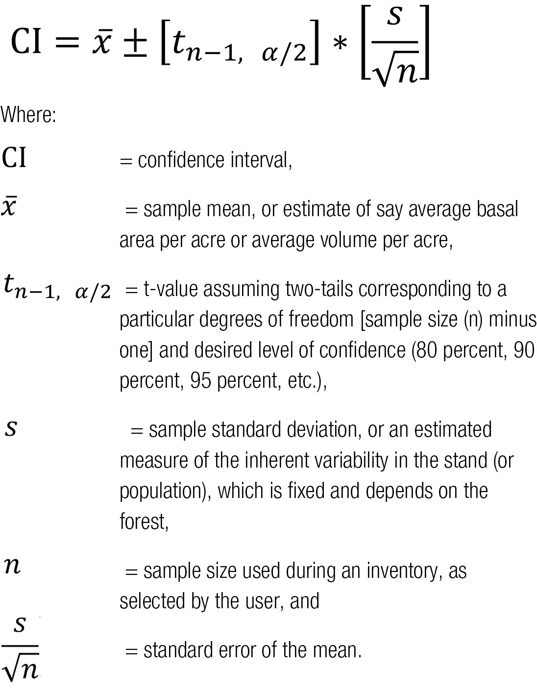
Notice a few things in the equation. The inventory sample size (n) is in the denominator. Based on sampling theory, this equation has built into it that, as sample size increases, the interval around your estimate, which likely contains the true average value, will decrease. Thus you can have more confidence in your estimate. This makes sense. Once again, you choose sample size.
The amount of inherent variability, or the variability among your plot/point estimates, is in the numerator represented by the standard deviation (s). As your standard deviation increases, for the same sample size, you should have less confidence in your estimate, which makes sense. Once again, the amount of inherent variability is fixed; it cannot be changed.
Finally, the t-value is a function of sample size (n) and your desired level of confidence. Do you want to be 80 percent, 90 percent, or 95 percent confident? As your desired level of confidence increases, the t-value will need to be larger to better account for all the uncertainty associated with your estimate of the average value, as well as the estimate of the standard deviation. You select your degree of confidence. The t-value is in the numerator, where a theoretical value of 1 is in the denominator:
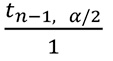
As the t-value increases, so does the width/size of the confidence interval.
Notice, though, that sample size in a sense has two impacts: one directly on the standard error of the mean and the second on the t-value. As your sample size increases, the t-value becomes smaller, eventually approaching the z-value corresponding to your desired level of confidence.
Statements of Probability Concerning Confidence Intervals
Remember that there is no probability associated with the true average value (or the parameter). The true average basal area or true average tons per acre is fixed at a particular time. It doesn’t change given your sample size, sampling protocol, etc. If I conduct an inventory of a stand, and another person conducts an inventory of the same stand, the true average value is the same. What will change between these inventories are our estimates of that true value, the sample standard deviation, and our calculated confidence intervals. Once again, because we will be measuring a different reduced portion of the population (or stand), that will lead to different estimates. For the three spatial layouts of five plots depicted in the pictured stand, is the true average value different between the three spatial layouts? No, the same stand is being sampled, but what is different among the three spatial layouts is the reduced portion of the stand that is being measured. Consequently, what does differ is the estimated average value and other associated sample statistics.
To say there is a 95 percent chance that the true average basal area is within some interval is technically incorrect. Notice you are putting the probability on the true value, whether I use a sample size of 12 plots or 50 plots, the true average value is the same. The change occurs in the confidence intervals. Therefore, the probability should be placed on the confidence interval, not the true average value.
It would be correct to say something similar to “There is a 95 percent chance that this confidence interval contains the true average value.” Notice, you are putting the probability on the interval (a statistic), not the true average value (a parameter).
Publication 3829 (POD-10-22)
By Curtis L. VanderSchaaf, PhD, Assistant Professor, Central Mississippi Research and Extension Center. Paul Doruska, PhD, Professor of Forest Measurements, College of Natural Resources, University of Wisconsin-Stevens Point; and Krishna Poudel, PhD, Assistant Professor, Department of Forestry, Mississippi State University provided useful comments.
The Mississippi State University Extension Service is working to ensure all web content is accessible to all users. If you need assistance accessing any of our content, please email the webteam or call 662-325-2262.