Setting Effective Rates for a Public Water System

Board Member Responsibilities

As a board member governing a public water system, you are responsible for the health and safety of the system’s customers. If you are a board member for a water association or a small municipality, you would have learned about these types of issues in the Board Management Training for Officials of Public Water Systems.

The responsibilities of a public water system board member fall into three primary areas, including:

• providing a safe and affordable supply of water to the system’s customers;
• communicating with the system’s customers; and
• ensuring that the system is operating on a sound financial basis for future sustainability.

This publication will focus on the last concept, while at the same time helping governing bodies of public water systems consider all relevant factors of financial sustainability when reviewing rate structures. People purchasing water must know that their water is safe and that it is provided as economically as possible without jeopardizing the future of the water system. While developing a rate structure that will accomplish these goals, the governing board must remember that there are several stakeholders that will influence the financial health and sustainability of the system. These stakeholders include:

• customers
• employees
• lenders
• regulatory agencies
• local, regional, and state elected and non-elected leaders (much of the influence of this group of stakeholders depends on whether the system is a municipal system or a water association)

Financial Sustainability

The concept of financial sustainability is extremely important for the sustainable operation of a public water system. Sustainable financial management provides the monetary resources necessary to enable a system to operate safely, update and upgrade treatment and distribution facilities, and perhaps even expand to serve more customers. The main purpose of the board’s existence is to provide its customers with an abundant and consistent supply of good-quality water at a fair and reasonable price. A primary board function involves adopting strategies that will allow the system to continue to provide safe water to its customers, including managing the finances of the system. Although a rural water association or a small city water service department is a nonprofit entity, it must be managed with the same scrutiny of a private business.

The American Water Works Association provides a five-factor process by which a quality rate structure, along with appropriate rate levels for the specific system, can be developed. These developmental steps include:

• Determine the revenue requirements of the system to cover the true or total cost of water.
• Develop a rate structure and rate levels to ensure that the system is financially sound and sustainable.
• Use customer classes (residential, commercial, industrial, etc.) to develop appropriate rate structures and levels.
• Write policies (water associations) or ordinances (government-owned systems) that define the system’s rate requirements.
• Take all emotion out of setting rates.

What constitutes financial sustainability or even financial stability? These concepts depend on the perspective of the entity examining the system. A lender wants to make sure that the system has sufficient cash flow to make the loan payment. A waterworks operator wants to develop a contingency fund that can pay for emergency repairs as well as system expansions and upgrades. The conscientious board member recognizes these needs as well as others, including fair wages and benefits for employees, maintenance of the system’s cash flow and excess returns, and affordability for customers.

In the past, many systems relied on grants and loans to address these issues. However, grants are increasingly scarce and lenders of all types are requiring a system to have a sound financial strategy before they will provide the system with debt capital.

Board members need to take a much larger view. While the system’s cash flow (liquidity) is very important because it allows the system to pay its bills, the concept of solvency (having an excess return over all expenses) is just as critical. As the governing body of the system, the board is responsible for being concerned with all of these concepts, and they owe it to their customers to manage the system according to these principles.

All too often a board believes the only option to improve the financial situation of the system is to adjust (usually raise) rates. While raising a system’s rates is certainly one way of increasing income to meet operating and capital expenses, it is not the only way. An appropriate rate structure and rate levels are essential to the financial sustainability and stability of the public water system, but there are other factors that can also contribute to the financial strength of the system.

Systems should ensure that the water meters being used to bill customers register the flow of water as accurately as possible. Because the water system makes money by billing for water flowing through customers’ meters, the system should be in working order to benefit both customers and providers. Bear in mind that a meter will over-read only in extremely rare circumstances. For the most part, a meter begins to age and lose accuracy (begins to record lower and lower usages over time) on the day that the meter is installed. Meters that do not accurately record the flow of water place an additional financial burden on the system and its customers.

For example, if a connection actually uses 5,000 gallons of water per month but the meter is only registering 80 percent of the water flowing through it, then the customer will be billed for only 4,000 gallons. This means that the customer receives almost 2.5 free months of usage over the course of the year. This situation puts an undue burden on the system’s other customers to cover the cost of the 1,000 gallons that didn’t register on the meter.

Systems should also adhere to strict and effective collection policies. As with aging meters, water systems must cover the cost of water that is delivered without receiving payment. Collection policies should implement a monetary penalty (i.e., late charge) that will discourage nonpayment habits. Systems should also implement a fair and strict cut-off policy with relatively large reconnection fees to discourage nonpayment. Systems should set reconnection fees at a level high enough to discourage repeat offenses, but not so high that customers either can’t pay the fee or refuse to pay the fee.

Systems may conduct water audits to identify areas where policies can be revised to either reduce the expenses or increase the income of the system to become or remain financially stable. For example, new connection fees and service fees should be structured to recuperate all necessary costs of labor and materials, in addition to providing another source of revenue for the system. Though these types of fees should not be the sole means to to having a sustainable system, funds generated by these fees can help offset utility-related expenditures.

Adjusting rates should be done as a last resort and only after the board has a complete understanding of the true or total cost of treating and distributing water and has performed a thorough examination of the system’s financial picture. There are several issues that should be considered before adjusting rates:

• Raising rates because of inefficiency and poor management is unfair to customers. Poor management cannot be overcome by raising rates. A loss of confidence and support from customers will occur, often resulting in the failure of the existing organization or leadership.
• Second, consider the level of water loss and unaccounted-for water. The majority of water loss can usually be attributed to two areas: inaccurate meters and leaks in the distribution system. When customers discover and report leaks to the system’s management or operations personnel and nothing is done to repair these leaks, then customers rightfully feel that management cares little about supplying water in a cost-effective manner.
• Other factors to consider when contemplating rate adjustments include decreases in customers’ personal incomes (often resulting from job losses) and people moving out of the district. These may be problems even under the best management conditions.

Simply, a basic rule of financial sustainability is that revenues must exceed expenses on a continuing basis. This can be accomplished either by managing expenses or by managing revenues. The most successful systems maintain financial sustainability through an efficient balance between the two. The remainder of this article will focus on the concept of revenue management, particularly as it relates to the system’s rate structure.

 

Role of the Rate Structure in Financial Sustainability

The rate structure is the financial engine that keeps the water system organization in business. The boards of directors and managers of small rural water systems are not only responsible for the system operating as efficiently as possible, but also for generating enough funds to meet normal expenses, emergency needs, and the long-term viability of the system through capital investment. If a thorough examination of the system’s finances indicates that a rate adjustment is in order, then the system should look at both its rate structure and rate levels to ensure that its long-term goals and objectives can be met. It isn’t enough for a system to simply “break even” in its business operations. Systems must also be financially prepared to pay for expenses over which they have little control. Rates should be set based on actual expenses of the system, depreciation, and future system needs.

Consideration should also be given to the impact of certain rate structures on individual users. Systems with primarily fixed-income/low-usage customers will not be as successful with certain types of rate structures as systems with a large percentage of higher-income/high-usage customers. Systems that serve many households with large, manicured yards or pools will have more fluctuation in usage between summer and winter months than urban systems where usages do not vary a great deal. During the summer, systems may have to compensate for customers using large amounts of water for discretionary uses (lawn maintenance, filling pools, watering large gardens, etc.). Regardless of the type of rate structure, systems must be mindful of the impact a bill increase will have on fixed-income customers and ensure fairness for all customers.

 

Basis of the System Rates and Rate Structure

System rates and rate structures should always be derived from the system’s projected costs. Think about the total cost of providing water to customers as being divided into three categories:

• projected levels of current operating costs (excluding capital costs)
• projected levels of future planned costs (typically capital improvements or expansions)
• projected levels of unplanned costs (unforeseen equipment failures)

The current level of these costs can be obtained from two important financial statements. The profit and loss statement (also referred to as the income statement) shows the expenses incurred. The cash flow statement shows the system’s cash outlays. While these statements are very similar (particularly if the profit and loss statement is generated on a cash basis)¹, there are two important distinctions. First, principal repayments on debt service are not counted as expenses to the system (remember that loan proceeds are not counted as income) and will not appear on the profit and loss statement. Second, depreciation is a noncash expense resulting from the use and obsolescence² of capital equipment. As a noncash expense, it does not appear on the cash flow statement.

Throughout the remainder of this publication, we will use a hypothetical 600-connection system that sells approximately 32 million gallons of water per year as an example to demonstrate the various concepts regarding the development of a rate structure. Table 1 contains the profit and loss and cash flow statements for our example. In this example, the profit and loss statement has been generated on a cash accounting basis.

Table 1. Example firm profit and loss and cash flow statements.

Description	Profit and loss statement	Cash flow statement
Operator Services	$54,748	$54,748
Operating Supplies	$11,793	$11,793
Repairs/Maintenance	$17,548	$17,548
Utilities	$19,821	$19,821
Contractual	$15,678	$15,678
Insurance	$3,500	$3,500
Miscellaneous Expense	$1,500	$1,500
Office Expense	$12,432	$12,432
Interest Expense	$26,800	$26,800
Principal Payments	$0	$116,900
Depreciation Expense	$68,276	$0
Total Expenses/Outlays	$221,060	$277,466

 

Projected Levels of Operating Costs
(excluding capital costs)

While determining the levels of operating costs that should be included in the rate structure, it is necessary to examine one of two financial statements. Both the profit and loss statement (particularly if it is generated on a cash accounting basis) and the cash flow statement will provide a comprehensive list of operating outlays that must be covered by the rate structure. If the profit and loss statement has been generated on a cash basis, these statements will be identical regarding operating costs with the exceptions of debt principal payments and depreciation expenses. If the profit and loss statement is generated on an accrual basis, there will be some difference (though likely not significant) due to expenses being recorded when they occur rather than when they are paid.

Table 2 shows that our rates need to cover $137,020 in operating expenses for the current year. However, it is likely that these expenses will increase for the next year. The important question is, “How much of an increase should be allocated?”

 

Table 2. Operating expenses.

Description	Current year P&L statement	8% projected increase
Operator Services	$54,748	$59,128
Operating Supplies	$11,793	$12,736
Repairs/Maintenance	$17,548	$18,952
Utilities	$19,821	$21,407
Contractual	$15,678	$16,932
Insurance	$3,500	$3,780
Miscellaneous Expense	$1,500	$1,620
Office Expense	$12,432	$13,427
Total	$137,020	$147,982

 

Many systems use the inflation rate reported by the federal government when looking at the level to increase projected costs. However, remember that this inflation rate usually is an average of the increase of the prices of all goods that consumers purchase. When dealing with relatively small-scale production processes, it is likely that operating costs will increase more than inflation. Therefore, let’s assume that we expect these costs to increase by 8 percent. This suggests that we should expect $147,982 in operating costs that should be covered by our rate structure.

Note that no interest costs appear in this section of the profit and loss statement. This means that the system does not have an operating loan in its debt financing portfolio. If this type of loan did exist, then the interest and principal payments would need to be included in the determination of operating expenses and outlays that would need to be covered by the rate structure.

 

Projected Levels of Future Planned Capital Costs

The next set of costs to examine are the current and planned capital costs. An obvious component of these costs that must be funded by the rate structure is the debt service (principal repayment and interest payments) associated with any outstanding loans. Since most loans are structured with a constant payment, these outlays will likely not change from year to year.

However, these are not the only considerations when covering capital equipment costs. There are two aspects of these costs that should be considered when defining the rate structure. The first is the replacement of the current stock of capital equipment as it becomes obsolete or wears out. The original cost of the system’s capital equipment is captured in the depreciation schedules assigned to each piece of equipment. It would also be captured in the sum of principal repayments for debt service if no down payment was made at the time of the purchase of the equipment and the equipment was purchased using debt financing.

Using either depreciation or principal repayment is an excellent start for planning the replacement of capital equipment, but remember that principal payments made before the beginning of this effort as well as accumulated depreciation (depreciation that has been charged to the equipment before the planning cycle) must be recognized as being part of the original cost of equipment.

Using an example that will be tied to our 600-connection system, assume that a set of capital assets were purchased and put in service 5 years ago³. Assume that the following conditions are true:

Original asset purchase price	$1,195,100
Original loan amount	$1,195,100
Time in service	5 years
Interest rate	3.5% with annual payments of $143,700
Life of loan	10 years
Depreciable life	20 years
Depreciation method	MACRS4
Remaining useful life	20 years

 

Given these parameters, the depreciation expense for year 5 is $68,276 with $284,709 charged to accumulated depreciation in years 1–4. Also, the annual payment for the loan is $143,700. In year 5, $26,800 was paid as interest on the loan and $116,900 was the principal repayment for that year. Loan records reveal that the principal repayment for years 1–4 totaled $429,384. The entire depreciation and loan amortization schedules for the example system can be found in Appendix 1.

Given this scenario, two separate factors need to be included in the rate structure. First, as previously mentioned, the annual loan payment (including principal and interest payments) of $143,700 is an obvious current obligation of the system.

Second, these assets will likely have to be replaced and perhaps even upgraded in 20 years (the end of the useful life of the assets). This is a projected cost of the system and should be included in the rate structure. We know that the original purchase price of the equipment 5 years ago was $1,195,100. After checking with equipment suppliers, we discover that the asset would cost $1,350,000 if we were to replace it today. We can see that the price of the asset has increased an average of about 2.6 percent per year.

However, we believe this equipment will need to be upgraded when it is replaced in 20 years’ time. Our equipment suppliers reveal that the current cost of the upgraded equipment is $1,500,000. An acceptable method of estimating the future cost of the upgraded equipment is to apply the 2.6 average annual percentage rate increase for 20 years to the current upgraded equipment cost of $1,500,000. This provides a future price estimate of $2,506,330⁵.

The governing board must decide on a strategy to fund this future purchase. There are three options that the board may pursue:

• Add nothing to the rate structure and depend on a future loan of $2,506,330.
• Include the total future purchase price in the rate structure and borrow nothing when it is time to replace the equipment.
• Include a portion of the future purchase price in the rate structure and borrow the remainder at the time of purchase.

After careful deliberation, the board decides that the third option is the best course of action for this particular circumstance. It is determined that 40 percent of the purchase price should be included in the rate structure and approximately 60 percent of the purchase price should be covered by a future loan⁶. This means that an average of $50,127 should be collected and allocated to the future purchase of these assets each year (an average of $4,177 per month)⁷.

The other component of planned future capital purchases closely follows this same reasoning. These are planned capital purchases for which there is no outstanding loan. Let’s assume that the system’s asset management plan indicates that a new pump motor needs to be installed in 4 years. Suppliers indicate that the current price of the motor (including installation) is $40,000 and that the prices increases by 3 percent per year. Using our previous logic, the future purchase price of the motor is $45,000, and the board wants to develop a rate structure that will pay for the motor with no debt financing. This suggests that the rate structure should accrue approximately $11,400 per year ($950 per month) to fund the purchase of the motor.

 

Projected Levels of Unplanned Costs (unforeseen equipment failures)

The final costs to examine are unplanned costs to the system that often result from capital equipment failure. While these types of costs can often be mitigated with an effective asset management plan, there are times when unforeseen circumstances occur. Furthermore, the level of these costs can be catastrophic to the system.

While the level of these costs cannot be accurately predicted, many water systems try to build a reserve or contingency fund over several years to provide protection from large costs. While some water systems allow their contingency fund to increase by whatever amount they have left over at the end of the year, systems with a strategic financial management plan typically have a goal to increase this fund by either a set amount each year or by a percentage of their revenue or total expenses.

For our example system, we will allocate 15 percent of the total expenses of the system for the current year (operating expenses plus interest and depreciation) to be set aside for the contingency fund. With projected annual operating expenses for the next year of $147,982, interest expenses of $26,800, and depreciation expense of $68,276, we want to design our rate structure so that it will generate $24,305 that can be allocated to this fund.

Given the data contained in these three cost categories, the rate structure and rate levels that are chosen for this example system will need to generate $377,514 in annual revenue to cover the following costs:

• $147,982—projected annual operating costs
• $50,127—planned equipment upgrades
• $11,400—planned pump motor replacement
• $143,700—debt service
• $24,305—contingency fund

 

Rate Structure Considerations

There are typically three areas of concern that a water system should address when considering the development of a rate structure. First, does the structure have the ability to generate the revenue necessary to cover the system’s fixed and operating expenses? If not, then it should not be considered as a viable option. It is important to remember, however, that these costs include more than just the system’s current operating obligations such as debt service, salaries, and treatment chemicals. They also include the depreciation of capital assets, accumulation of funds for future capital improvements, and emergency reserve or contingency funds.

Second, does the structure contain an incentive to conserve water? Water is a precious natural resource that is required for sustaining life. A rate structure that does not provide an incentive for customers to conserve water is likely falling short of a major goal.

Finally, is the rate structure “fair” to different classes and levels of users? In the simplest terms, the total amount that customers are charged for each billing period (usually a month) should be directly related to the amount of water that they consume. This does not mean that each customer should pay the same total bill for water or that they should pay the same price per gallon of water consumed. Rather, it suggests that if Customer A consumes more water than Customer B, then Customer A should pay a higher bill. The system’s rates should be designed so that no particular customer class or group is subsidizing another class of customer.

This issue of fairness may be most effectively demonstrated with “effective rates” as opposed to “stated rates.” Stated rates are published by the system to its customers and describe the “rules” for calculating a particular customer’s total bill. The effective rate is the total bill divided by water consumption (usually expressed in thousands of gallons)⁸ and describes the actual amount that the customer is being charged per unit of water consumed.

 

Requirements for Effective Rate Structures

Above all, remember that defining an effective rate structure for a public water system requires accurate cost and revenue data. To obtain accurate cost data, it is important to classify the expenditures and other financial outlays of the system in a manner that makes it possible to perform an accurate cost analysis (remember, the first goal of the rate structure should be to recoup the system’s costs). This requires the system to invest a significant planning effort in its record-keeping system to ensure consistency in the record-entry process. Without consistency, the system’s cost records will not provide accurate information to guide the rate structure decision-making process.

Just as important is accurate revenue (billing) data, particularly if a system is facing tight financial constraints and must closely monitor monthly cash flow. Most systems use some type of billing software to generate bills for customer usage, and this is the key source of information for determining the appropriate rate structure and levels. However, this software has to have accurate information if the output is to be useful.

Meters should be regularly checked to ensure that they are providing accurate readings. If the system charges a different rate based on connection size, then this information must be accurately recorded in the billing software. Also, meters must be read on an accurate and consistent basis. Accuracy means that the actual meter reading must be recorded; “penciling readings,” or guessing the reading for a particular billing cycle, will corrupt the data and lead to making decisions based on false data. Consistency means that the meters should be read as closely as possible to the same date for every billing cycle (the billing cycle is typically monthly, but some meters may be read on a quarterly, seasonal, or even annual basis).

Rate Structure Definitions

With few exceptions, the public water system’s primary source of revenue is a result of the rates that govern the amount that customers pay for their consumption of water. While the total amount of revenue earned by the system may be the primary goal, the rate structure and rate levels that govern how this revenue is collected are of equal importance. Remember that rates should be structured so that each customer pays a “fair” share for the water consumed; this means that no one should pay any more or any less than their equitable contribution to the system. This does not mean that every customer’s bill should be exactly the same; rather, each customer’s bill should be related to the amount of water consumed.

Once the system’s expenses have been identified, a rate structure can begin to be developed. The typical water utility rate is based on two separate components. First, the base minimum is typically a component of all rate structures. The customer pays a fixed amount for consumption of a set amount of water or less. For example, the base minimum might be $25 for the first 2,000 gallons of water; if a customer only consumed 750 gallons for a particular month, the bill would be $25 for that month. This minimum covers a major portion of a system’s costs and historically has been designed to generate income adequate to cover the fixed expenses of a system.

The second component of all rate structures (except for the flat rate structure) is the flow rate. The flow rate is charged for each additional unit of water (usually measured in thousands of gallons) over the base minimum amount. For example, after the first 2,000 gallons are used, the customer may be charged $6 for each additional thousand gallons of water used.

 

Flat Rate Structure

The flat rate structure is the most basic type of rate structure and has the advantage of being the simplest for a system to administer. Flat rate structures charge every customer the same amount for water each month regardless of how much is used. For example, consider a system that has a flat rate of $25 per month. A household using 2,000 gallons and a household using 6,000 gallons are both charged $25 under this type of structure. However, flat rate structures have several disadvantages. These types of structures encourage waste, tend to be unfair to different customer categories, and often do not provide the necessary income to cover expenses.

If we apply a flat rate structure to our 600-connection example, the monthly charge would be calculated by dividing the level of costs that need to be covered ($377,514) by the number of customers (600) to get the annual bill per customer ($629.20). This amount would then be divided by 12 months to obtain the per-customer bill (approximately $52.50 per month). However, this rate structure falls short of all the important considerations mentioned above.

First, since there is no additional charge for consuming higher quantities of water, there is no incentive to conserve water through such basic actions as fixing leaks and turning off garden hoses. Second, our costs are based upon the sales of 30 million gallons per year; increased waste will result in increased water production and, therefore, increased operating or variable costs. This rate structure will likely not generate the revenue necessary for the system to cover its costs.

Finally, it is unlikely that this rate structure can be viewed as being fair to all customers. Table 3 demonstrates the total bill and effective rate (per 1,000 gallons consumed) for different levels of usage. Remember that the effective rate can be viewed as a measure of the fairness of the rate structure.

 

Table 3. Flat rate structure.

Usage (per 1,000 gallons)	Total bill	Effective rate
1,000 gallons	$52.50	$52.50
2,000 gallons	$52.50	$26.25
5,000 gallons	$52.50	$10.50
10,000 gallons	$52.50	$5.25
20,000 gallons	$52.50	$2.63

 

As can be readily seen, low-volume users pay an inordinately high rate per 1,000 gallons of water consumed as compared to high-volume users. It is obvious that this rate structure is not very fair to customers of lower usage levels.

Uniform Block Rate Structure

The uniform block rate structure with a minimum base is likely the most common rate structure used in Mississippi. Uniform block rate structures typically have a base minimum rate and a flow rate that does not vary with the level of consumption.

There are several methods that can be used to determine the specific rate levels associated with this structure. The final levels will likely encompass factors of all methods.

The first and most traditional method involves covering the fixed expenses of the system with the base minimum rate and then using the flow rate to cover the system’s variable expenses. In the 600-connection example, the annual fixed expenses would be comprised of the planned equipment upgrades ($50,127), the planned pump motor replacement ($11,400), and the annual debt service ($143,700) for total fixed expenses of $205,227. Using the same logic as in the fixed rate structure section above, each customer would have a base minimum of $342.05 per year, or about $28.50 per month⁹. The governing board would need to make a determination of the number of gallons that would be included in the base minimum; for this example, this level of consumption will be 2,000 gallons.

The variable expenses to be covered by the flow rate that affects consumption above the base minimum would include the current operating expenses ($147,982) and the contingency fund ($24,305)¹⁰. Using the individual usage patterns of the customers in the example system, the flow rate would need to be approximately $7.50 for each 1,000 gallon block of water consumed over the initial 2,000-gallon base minimum.

The other method involves setting a base minimum rate that the board feels is fair or equitable to low-volume customers and then using the flow rate to cover the difference in expenses. There is some risk in using this method. If the base minimum is lowered, then the system is depending on variable usage to cover fixed costs. In years with a substantial amount of rainfall, water consumption may decline to the point where fixed costs are not covered.

If the base minimum is increased, then fixed revenue is used to cover variable costs. In dry years, water consumption may increase to the point where these variable costs may not be covered. If this method is to be used for the example system and the board decided to lower the minimum base to $25 for 2,000 gallons, then the flow rate would need to be increased to about $8.60 per 1,000-gallon block.

When compared to the flat rate structure, the uniform block rate structure does a better job of addressing important considerations. Since there is an additional charge for consuming higher quantities of water, there is an incentive for customers to conserve water through such basic actions as fixing leaks and turning off garden hoses. Second, since the flow rate is based on the variable costs projected to be incurred by the system, increased water use will result in increased revenue sufficient to cover these increased variable costs.

Finally, this rate structure is fairer to customers than the flat rate structure as shown by the effective rate measure. Table 4 shows the total bill charged to specific user levels and the effective rate per 1,000 gallons for the usage level given a $28.50 base minimum with 2,000 gallons of usage and a $7.50 per 1,000-gallon block flow rate.

 

Table 4. Uniform block rate structure with a base minimum.

Usage (per 1,000 gallons)	Total bill	Effective rate
1,000 gallons	$28.50	$28.50
2,000 gallons	$28.50	$14.25
5,000 gallons	$50.00	$10.00
10,000 gallons	$88.50	$8.85
20,000 gallons	$168.90	$8.45

 

The effective rate for a 5,000-gallon user is approximately the same under the uniform block rate structure as for the flat rate structure, and the effective rates for high-volume users are much higher under the uniform block rate structure. However, the effective rates for low-volume users are much lower under the uniform block rate structure. While it is obvious that the effective rate declines as usage increases, the range of effective rates across usage levels is much smaller for the uniform block rate structure than for the flat rate structure.

Decreasing Block Rate Structure

A decreasing block rate structure typically charges a base minimum, but each subsequent consumption block declines in price. If organized carefully, a decreasing block rate can adequately pay a system’s expenses, but it may not provide enough income to cover unexpected demands and future needs.

The base minimum for a decreasing block rate structure can be calculated in the same manner as that for the uniform block rate structure. While the base minimum has traditionally been determined by the level of the system’s fixed costs, it can also be adjusted by the board to provide a lower rate for low-volume users. However, the decreasing block rate has traditionally been used to attract high-volume users such as water-intensive industries.

Following our previous example, we will use the $28.50 minimum base for 2,000 gallons. If the board has decided that a $1 differential per consumption block above the minimum base is the policy that it wants to follow, then the following flow rates would be necessary to generate the revenue needed to cover the system’s variable costs:

 

Table 5. Example flow rates.

Usage	Flow rate change
2,001–3,000 gallons	$10 per 1,000 gallons
3,001–4,000 gallons	$9 per 1,000 gallons
4,001–5,000 gallons	$8 per 1,000 gallons
5,001–6,000 gallons	$7 per 1,000 gallons
6,001 gallons and above	$6 per 1,000 gallons

 

 

Table 6. Decreasing block rate structure with a base minimum

Usage (per 1,000 gallons)	Total bill	Effective rate
1,000 gallons	$28.50	$28.50
2,000 gallons	$28.50	$14.25
5,000 gallons	$55.50	$11.10
10,000 gallons	$86.50	$8.65
20,000 gallons	$146.50	$7.33

 

While Table 6 shows that the decreasing block rate structure does a better job of addressing the question of fairness in pricing than does the flat rate structure, there is a wider gap between the effective rate per 1,000 gallons of usage for low-volume and high-volume users than there is for the uniform block rate structure.

In our example, the base minimum was set at a level that recouped the fixed costs of the system, so the decreasing block rate is equivalent to the uniform block rate structure for this measure. However, the flow rates are set at a level that covered the variable costs of producing water for an annual production of 32 million gallons. In a wet year when water consumption declines, the decreasing block rate structure is likely to be more than adequate in covering these variable costs. However, in dry years when water consumption could increase substantially, the decreasing block rate structure could fall short in covering additional variable costs.

Since the price of consuming each additional block of water declines until a level of 6,000 gallons is reached, the decreasing block rate structure does not contain the level of incentive to conserve water as much as the uniform block rate structure (although the incentive to conserve is much greater than the flat rate structure). For all of the reasons mentioned, the decreasing block rate structure is typically not recommended to be used for residential rates.

However, this structure is often used for industrial or other commercial customers that have very high usage rates. There is an economic logic behind this decision. Many water systems with high production capacity experience “increasing returns to scale” in the production of water. That is, the average cost of water declines as the quantity of water produced increases. This declining production cost can fit nicely with the declining block rates in this rate structure.

 

Increasing Block Rate Structure

An increasing block rate structure typically charges a base minimum, but each subsequent consumption block increases in price. The base minimum for an increasing block rate structure can be calculated in the same manner as that for the uniform and decreasing block rate structures. As previously mentioned, while the base minimum has traditionally been determined by the level of the system’s fixed costs, it can also be adjusted by the board to provide a lower rate for low-volume users.

The increasing block rate structure is an excellent way to increase income for the system, since income increases at a faster rate as consumption increases. The increasing block rate structure encourages customers to conserve water and should not negatively affect most small households as compared to the uniform and decreasing block rate structures.

Following our previous example, we will use the $28.50 minimum base for 2,000 gallons. If the board has decided that a $1 differential per consumption block above the base minimum is the policy that it wants to follow, then the following flow rates would be necessary to generate the revenue needed to cover the system’s variable costs:

 

Table 7. Example flow rates.

Usage	Flow Rate Change
2,001–3,000 gallons	$5 per 1,000 gallons
3,001–4,000 gallons	$6 per 1,000 gallons
4,001–5,000 gallons	$7 per 1,000 gallons
5,001–6,000 gallons	$8 per 1,000 gallons
6,001 gallons and above	$9 per 1,000 gallons

 

 

Table 8. Increasing block rate structure with a base minimum.

Usage (per 1,000 gallons)	Total bill	Effective rate
1,000 gallons	$28.50	$28.50
2,000 gallons	$28.50	$14.25
5,000 gallons	$46.50	$9.30
10,000 gallons	$90.50	$9.05
20,000 gallons	$180.50	$9.03

 

 

Table 8 shows the effects of the increasing block rate structure described above on the customer’s total bill and effective rate per 1,000 gallons of consumption for various usage levels. Note that while the effective rate initially declines, it begins to increase at a slow rate as consumption increases above 5,000 gallons. In terms of pricing fairness, the gap between the effective rate for low-volume and high-volume users is the narrowest with this rate structure. Also, this type of rate structure would likely cover the variable (as well as fixed) costs of the system no matter the level of total water production.

However, this type of rate structure does not encourage economic development. Large households and high-volume consumers such as certain businesses and industries (e.g., food processing plants) will have relatively high bills due to higher consumption of water. If a water system is contemplating an increasing block rate structure, it will often apply this structure to residential users and use either a uniform or decreasing block rate structure for commercial and industrial customers.

 

Comparing the Rate Structures

In terms of comparing the four rate structures, there is little doubt that the flat rate structure is the poorest performing of all. While it is the simplest structure to implement, it fails the other effectiveness tests. It provides no incentive for water conservation, will likely not provide the level of revenue necessary to cover variable costs in times of above-average usage, and has the largest gap in the effective rates of low- and high-volume users.

The three block rate structures have various strengths and weaknesses. In terms of conservation incentives, the increasing block rate structure is the strongest, followed by the uniform block rate structure and then the decreasing block rate structures. However, the decreasing block rate structure is the most conducive to economic development by requiring lower input costs for businesses and industries that use high volumes of water.

The increasing block rate structure is the most likely to be able to cover the variable costs of the system, particularly in years of high water usage. The same logic suggests that the decreasing block rate structure may very well prove to be the most effective in covering variable costs in low usage years. Also, the increasing block rate structure has the best ability to generate a significant amount of revenue in a fairly short time.

In terms of pricing fairness, the increasing block rate structure tends to provide the narrowest effective rate gap between low- and high-volume users, followed by the uniform block rate and the decreasing block rate structures.

There are two other factors that should be considered, as well. The first is the ability of the system’s customers to understand the particular rate structure that has been chosen by the governing board. The uniform block rate structure is easy to understand: every user that consumes more than the base minimum pays the same cost for each additional consumption block above the base minimum consumption level.

The decreasing block rate structure is likely the least understood structure by the customers, particularly low-usage residential customers. These customers typically have difficulty understanding why a high-volume customer should pay a lower rate for each consecutive block of consumption. This difficulty, coupled with the fact that most low-usage residential customers tend to have low or fixed incomes, provides another reason why the decreasing block rate structure is usually reserved for high-volume businesses and industries.

The other factor concerns the determination of the rate levels necessary to cover the expenses of the system when taking user patterns into account. While this may seem to be a difficult concept to understand at first glance, it becomes quite clear when the example rate structures from the example system are examined.

Initially, one might suppose that the rate levels for the increasing block rate structure should be the mirror image of the rate levels for the decreasing block rate structure. Also, it seems intuitive that the level of the uniform block rate structure should be the average of the block prices for either the increasing or the decreasing block rate structure. This would be the case if the usage patterns of the system’s customers were symmetrical from the lowest user to the highest. However, this is seldom, if ever, the case for any water system.

Figure 1 shows the average monthly consumption graph for the example system. This graph shows that almost 50 percent of the system’s users consume 4,000 gallons of water or less per month and just over 72 percent of the users consume 6,000 gallons of water or less per month. Most small rural systems (regardless of whether they are municipalities or water associations) follow this same pattern. Therefore, the bulk of the system’s expenses must be paid by the low-volume users, particularly when the average volume of the highest-consumption customers (17,845 gallons for this example) tends to be relatively low.

Figure 1. Example system—average customer monthly consumption.

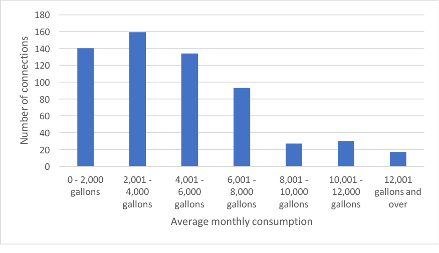
This means that the rate structure levels for the low-volume users must be relatively high, particularly when they are compared to a large system with a much higher percentage of high-volume users such as water-intensive businesses and industries or large-volume residential users.

 

Base Minimum vs. No Base Minimum

As has been mentioned, the base minimum represents a charge to the customer that is paid to the system regardless of how much water is used. Systems have traditionally used the base minimum to cover the system’s fixed expenses such as debt service, salaried employees, insurance, and future improvement or expansion plans.

A rate structure that includes a base minimum maintains a more level income stream over the course of the year. There are, however, several water systems that do not use a base minimum in their rate structure and only use a higher flow rate than would have been necessary if the base minimum had been used. This means that their income will vary greatly depending on usage, and usage will depend on the season or weather. In most cases, systems that do not have a base minimum in their rate structure must be prepared to cover their fixed costs from financial reserves during seasons or months when usage and, therefore, income is relatively low.

Systems that successfully forego using a base minimum in their rate structure tend to have several characteristics in common. These include:

• The system is in excellent financial condition.
• The system has an adequate level of financial reserves to carry it through prolonged low-usage periods.
• The system’s management uses effective financial management techniques.
• The system contains a relatively large number of high-volume users.

 

Figure 2 shows the example system’s monthly usage, the monthly revenue earned by the system under the uniform block rate structure with a base minimum as discussed above, and a uniform block rate structure without a base minimum but with a flow rate sufficient to cover the expense needs of the system (in this example, the flow rate used is $11 per 1,000 gallons of usage).

Figure 2. Comparison of the uniform block rate structure with and without a minimum base.

The top line in the graph represents the total monthly usage of the system. It is easy to see that both types of rate structures closely follow the usage pattern of the system (both rate structures are generating the same level of total annual revenue), but there are differences between the two.

While the level of revenue is higher for the rate structure without the base minimum component in high-use months, the reverse is true, as well. We can see from Figure 2 that the change in revenue from month to month is much larger for the rate structure without a base minimum, while the rate structure with a base minimum is much more stable.

 

Conclusion

Defining a rate structure and determining rate levels to ensure that a public water system is not only sustainable, but is also fair to all customers, is a difficult task for governing boards. Many factors must be considered. These include accuracy and consistency in the system’s financial management practices and an understanding of the system’s customers and their usage patterns.

The rate structure should be designed to cover the system’s true total cost, including depreciation, future capital asset replacements/improvements, and emergency or contingency reserves. If a system only covers its operating costs (salaries, supplies, utilities, etc.) and its debt service, it is not looking to the future and faces a declining net worth and decreased sustainability.

There are several types of basic rate structure designs from which the system can choose. The least effective of all rate structures is the flat rate structure. It fails to meet any of the criteria against which a rate structure should be tested except that of revenue stability.

The three block rate structures (uniform, decreasing, and increasing) have various strengths and weaknesses. The increasing and decreasing block rate structures usually tend to be reserved for certain user types. The uniform block rate structure is more accepted across a wide range of user classes, but it does not encourage economic development like the decreasing block rate structure, nor does it generate revenue as quickly or encourage conservation like the increasing block rate structure.

Any of the block rate structure types can be used with or without a base minimum rate. The omission of the base minimum makes water consumption more affordable for low-use customers, but it does result in a higher variation in the system’s income stream (particularly on a monthly basis). Furthermore, the system that adopts this type of strategy is depending on a variable revenue stream to cover its fixed expenses. This strategy tends to work best for systems that have high populations of relatively high-usage customers and that have sufficient cash reserves and financial management acumen to withstand prolonged usage periods (e.g., exceptionally wet seasons).

If a thorough examination of the system’s finances indicates that a rate adjustment is in order, then the system should consider the type of rate structures available, the level of rates, and the consumption patterns of the customer to ensure the financial stability of the public water system and meet its long-term goals.
 

Footnotes

¹ In a cash-based accounting system, income to the firm is recorded in the period in which cash is received from customers and expenses are recorded when the cash is paid out. In an accrual system, income and expenses are recorded in the period in which they are actually earned/incurred. While the accrual system typically provides a better picture of the financial health and stability of the firm, cash-based accounting systems are used by most water associations because of their ease of use. Municipalities will incorporate the accounting for a water system into the larger municipal picture and will likely use either cash-based or accrual-based accounting procedures, but not both (Averkamp).

² Obsolescence refers to capital equipment becoming obsolete and not suitable for use. The obsolete equipment may still “work,” but its function is no longer conducive to the system providing service in as efficient or cost-effective manner as possible.

³ This bundling of assets is used to keep the example as simple as possible. In practice, each asset would have to be examined individually to determine its depreciation expense, accumulated depreciation, and principal repayment.

⁴ https://www.irs.gov/publications/p946/ar02.html#en_US_2016_publink1000270861

⁵ This loan will be less than 40 percent of the future purchase price due to interest earned on additional dollars collected for the future purchase in the rate structure.

6Future purchase allocation =	$2,506,330 × 40%	= $50,127 per year
	20 years

⁷Contingency fund allocation = ($137,020 + $26,800 + $68,276) × 15% = $34,814

¹⁰ While many would classify some of the categories as fixed costs that this study has classified as variable costs (e.g., salaries and operator expenses), we have classified these as variable costs in order to maintain a reasonable level of both types of costs. Also, since the contingency fund is tied most closely to the system’s operating expenses, we will assume that it is a variable “cost” to the system.

 

 

References

Averkamp, H. Accounting Coach. https://www.accountingcoach.com/blog/cash-basis-accrual-basis-of-accounting.

American Water Works Association. (2004). Developing Rates for Small Systems: Manual of Water Supply Practices. Publication M54. Denver, CO. awwa.org.

 

Source: https://www.irs.gov/publications/p946/ar02.html#en_US_2016_publink1000270861

---

Publication 3172 (POD-12-17)

By Alan Barefield, PhD, Extension Professor, Agricultural Economics, and Lauren Behel, Extension Associate, Agricultural Economics.

Copyright 2017 by Mississippi State University. All rights reserved. This publication may be copied and distributed without alteration for nonprofit educational purposes provided that credit is given to the Mississippi State University Extension Service.